Simulation or Modeling of breakthrough curves
General information
Numerical simulations are useful tools for:
- The evaluation of experimental breakthrough curves in terms of determination of kinetic parameters
- A better understanding of the dynamic process
- Parametric studies
- Prediction of what is happening with a longer adsorbent packed bed, or different gas velocities
- The extrapolation or interpolation between experiments
- Reducing the experimental effort
The LDF approach
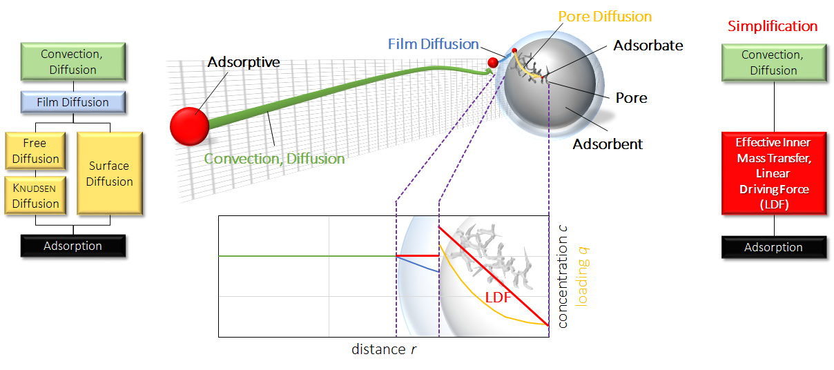
In most models, assumptions and simplifications are necessary to reduce calculation time and the number of unknown variables. In all calculations shown here, the linear driving force (LDF) assumption was applied. In the next figure this simplification is explained schematically.
Simplification of transport phenomena. The molecules have to travel gas phase through a thin film (blue) by convection or diffusion. In that thin layer, film diffusion is taking place onto the surface of the particle. Afterwards, the molecules have to diffuse in the porous particle to access the active sites. This can be achieved by surface diffusion, knudsen diffusion or free gas diffusion among others. By simplification, all these transport resistances are summarized in one overall parameter with an linear progress in concentration.
Further assumptions and simplifications
Beside the LDF-approach there are a lot of assumptions and simplifications in the applied model. Some of them are listed below:
- No mass, heat or velocity gradients in the radial direction
- No temperature gradient inside the particles and thermal equilibrium between the gas phase and adsorbent
- Ideal gas behavior
- Plug flow with axial mass dispersion
- No pressure drop along the fixed bed
- Negligible external mass transfer effect (i.e. film mass transfer and macropore diffusion)
- Negligible heat capacity of the adsorbed phase
- Heat capacity of carrier gas is dominating and constant
- Heat transfer resistances only on the inner surface and the outer surface of the wall, respectively
- Constant heat transfer coefficients
- Constant and homogeneous bed porosity along the bed length
The model consists of mass- and energy balances as well as an overall mass balance in case of variable gas velocity. All equations build a system of coupled differential equations which can be solved by a finite difference method. A detailed description of the model and the corresponding boundary parameters are given in research books of D.M. Ruthven, R.T. Yang and other researchers.
Input parameters for modeling
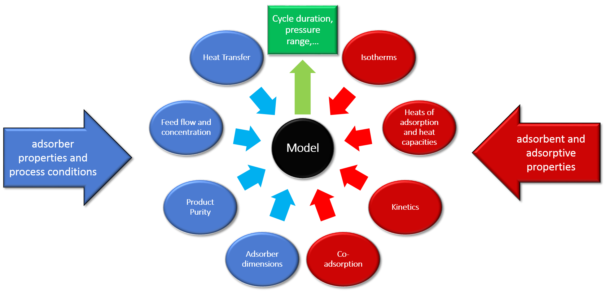
For a successful description of an experimental breakthrough curve under non-isothermal conditions, a couple of input parameters are needed:
- Properties of the adsorber (length, diameter, heat capacity of wall, wall thickness…)
- Experimental conditions (pressure, gas flow, inlet concentrations…)
- Properties of the adsorbent
- Isotherms of the adsorptive, described by an equilibrium model
- The temperature dependence for all parameters of the equilibrium isotherm model
- A starting value for the kinetics of the sorptive process (LDF-constant)
All necessary input parameters can be found in next figure.
Determination of LDF-constants
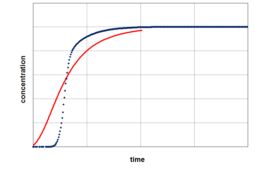
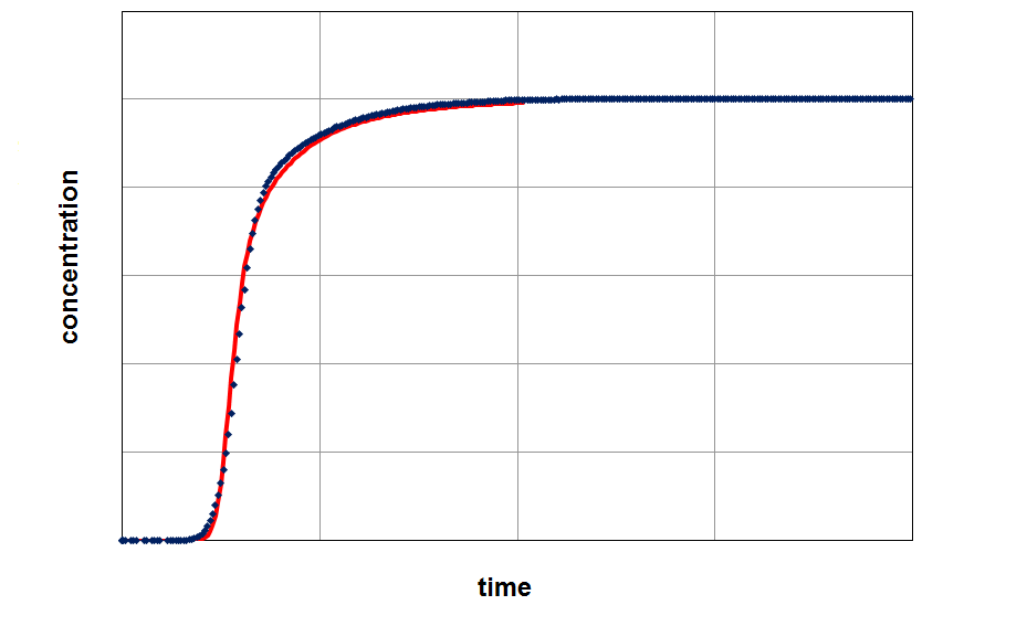
By fitting the model on an experimental breakthrough curve, one can estimate the LDF-constant for the system under investigation. On the left side the model was applied with a small, freely choosen LDF parameter. After fitting the model by variing of this parameter a better accordance between experiment and model can be observed (right part of the figure).
Applying the model (red curve) on experimental data (blue curve) with a randomly selected LDF-value (kLDF=1 1/min). In the example the isotherm with their temperature dependency was used as input parameter for modeling.
From the figures it is clear that a quantification of LDF-values is possible, if other input parameters for modeling are well known. This LDF-value can now used for comparison different adsorbents and further parametric studies and calculations with the aim of minimization of mass transfer zones can be performed.
Modeling of Adsorption and Desorption
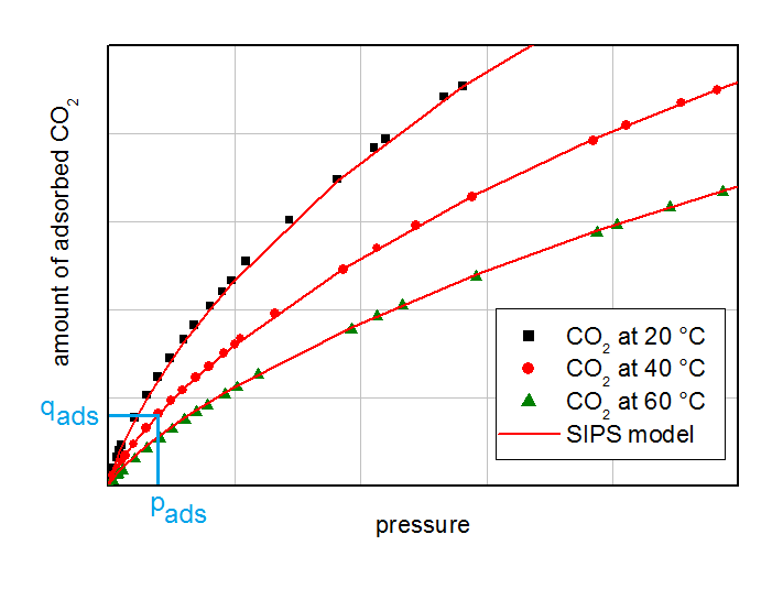
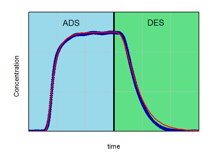
By modeling and/or measuring of adsorption and desorption the influence of the isotherm curvature can be investigated. In the next figure on the left side some isotherms on activated carbon are summarized. On the right side an adsorption/desorption experiment is showed. The breakthrough experiment was performed with 5 % CO2 in N2 on an activated carbon at 5 bar and 40 °C. Desorption was measured by flushing the equilibrated adsorber with pure Nitrogen. From the curved isotherms a favored adsorption was assumed. On the adsorption part in the right side of the figure a model was fitted to get the LDF-value for the next calculations. This LDF-value was held constant for calculating the desorption curve for later PSA-investigations.
Isotherms of CO2 on activated carbon. The partial pressure and the corresponding equilibrium loading for the breakthrough experiments are labeled with light blue lines.
The breakthrough experiments as well as the simulated curves show a lower desorption rate compared to the adsorption part. Therefore the desorption time by flushing with nitrogen will be longer as the adsorption time under same conditions. Further the total gas flow during desorption was the same as for the adsorption part. Under such conditions an enrichment of CO2 in the desorbed phase can be not achieved.
Calculations for PSA-experiments
Based on the model from the figure above, a simplified PSA-process was calculated. For this purpose, the desorption flow was set to 500 ml/min N2 in counter current, whereas the adsorption flow was 2000 ml/min (5 % CO2 in N2). The experimental adsorption time was obtained from the figure above with 5.75 min. The desorption duration was experimentally set to 5.00 min including the blow-down step. The pressurization step was 0.9 min with 2000 ml/min N2 in counter current flow and is shown as separate segment in the plots below. This step as well the blow down was not considered separately by calculations. The desorption time for calculations was set to 5.03 min. In all calculations the pressure release from 5 bar was implemented within the desorption step.
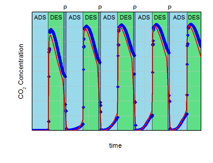
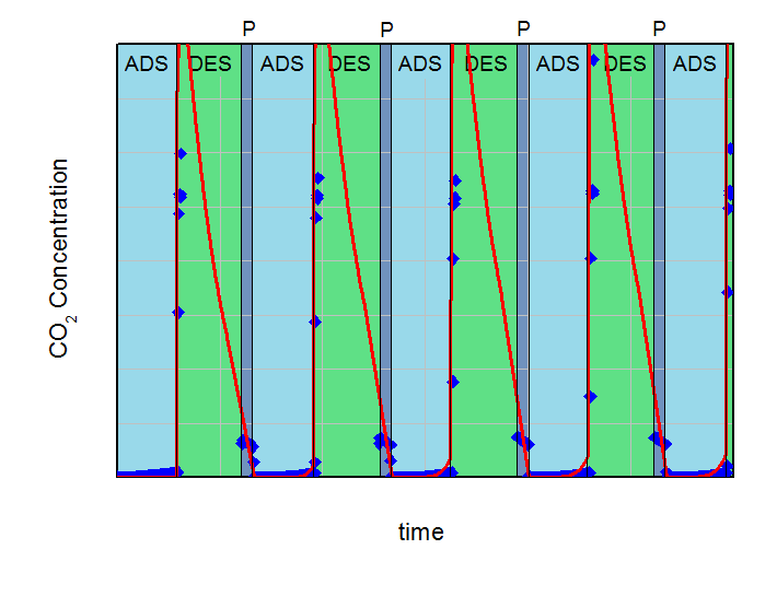
The aim of the calculations was to find the necessary desorption pressure for a breakthrough concentration below 1 % CO2 in the product flow during the adsorption step over five adsorption-desorption cycles. All results were compared to experimental data. Both, calculations and experiments are summarized in the next figures. On the left side the desorption pressure was set to 1 bar for all calculations. On the right side this value was reduced to 0.5 bar. For better comparison the y-axis and x-axis in both plots are identical.
Adsorption (ADS) with 2000 ml/min @ 5 bar and desorption (DES) with 500 ml/min @ 1 bar cycles with desorption in counter-current flow. Blue points are experimental results and red line are calculations. Pressurization is labeled with P.
In the left figure, an increasing effluent concentration of CO2 during adsorption with each cycle can be observed (build-up effect). This increase converged to approx. 2.3 % CO2 in the product after five cycles in the experiment and was in good agreement with the 2.7 %, predicted by the simulation. It is clear, that under the investigated conditions a desorption pressure of 1 bar is not low enough for a sufficient regeneration of the fixed bed adsorber. Contrary to that, the desorption pressure of 0.5 bar is sufficient for the necessary regeneration in the experiment as well as in the calculations. The concentration of CO2 in the product after five cycles was 0.84% for the predictive calculations and 0.18% for the experiment. These deviations between simulation and experiment can be explained with the simplifications of the model. However, this example shows how simulations can support finding of right parameterd for PSA-design and how to reduce the experimental effort considerably.
Modeling based on mass- and energy balances can help to understand the dynamic sorption process and is useful to reduce experimental effort by predicting important process parameters.

